
Start an analog comparison
- Open Analog field development in the application sidebar.
- Under Input mode, choose Describe prospect to enter your own parameters, or Existing field and select a Target field to populate its recorded depth and thickness values.
- Review the three target measurements, minimum history, number of analogs and activity cutoff in the sidebar.
- Click Analyze analog fields. Results load in stages: Wells, Oil and Gas, then Planned sites and APDs.
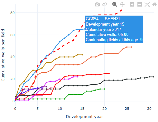
- Compare the field lines across the five charts. In Existing field mode, the target’s available history appears as a dashed red line without markers.
Changing analysis inputs clears earlier results. Click Analyze analog fields again to run the revised comparison. Each click refreshes the source data.
Choose the inputs
| Control | How to use it |
|---|---|
| Target water depth (ft) | Enter the prospect’s water depth. The ranking uses each candidate field’s recorded water depth. |
| Completion depth — top TVD (ft) | Enter a representative completion top true vertical depth. Existing-field values use the mean absolute completion top TVD of qualifying records. |
| Completion interval thickness (ft) | Enter the perforation interval length. Recorded field values average bottom minus top perforation measured depth; this is not necessarily true vertical reservoir thickness. |
| Minimum years of data | Default: 5. Require this many calendar years from first valid spud through the cutoff, inclusive. Intervening zero-activity years count. |
| Number of analog fields | Default: 10. Request the best qualifying matches. Fewer are returned when insufficient fields qualify. |
| Include activity through year | Use a completed calendar year. All five histories are included through December 31 of that year. The initial value is the configured cutoff or last completed year. |
All three target measurements must be positive. Analogs rank by the sum of relative differences in water depth, completion depth and interval thickness, with equal weight for each measurement. Lower scores mean closer matches. The minimum-history filter applies before ranking; the selected target field is excluded from its own analog set.
Read the five charts
| Panel | What it measures |
|---|---|
| Wells | Cumulative distinct well APIs spudded, including exploration and other well types with usable spud dates. This measures drilling starts rather than production starts. |
| Oil and Gas | Cumulative recorded oil in barrels and gas in Mcf. |
| Planned sites | Cumulative recorded planned sites, including available pre-spud activity. |
| APDs | Cumulative distinct well APIs with recorded applications for permits to drill, including available pre-spud applications. |
Development year 0 is each field’s own first-spud calendar year. A common x-axis aligns development ages rather than calendar dates. Hover for the field, development year, calendar year, cumulative value and contributor information.
The shared legend covers all five charts. Click a field name to hide or show it; double-click to isolate it. Click Average estimate to show the initially hidden dashed estimate, which accumulates mean annual additions using the fields observed at each development age. The target field is excluded from this estimate.
Logarithmic y-axis changes all five charts together. Only positive values can appear on a log axis; zero and negative values remain available in tables and CSVs. Development-year zoom is linked across the charts.
Use the map and workspace
Drag a panel header onto another panel to swap their positions. For keyboard operation, focus the header and use the arrow keys. Layouts stay with the current browser session, and panels stack on smaller screens. Hover over chart observations for details; use chart zoom and legend controls where available.
Tables and CSV downloads appear below the chart workspace. Expand the relevant table to see its contents. The dashboard’s method and data-quality guide is at the bottom.
Click a field observation or an analog field boundary to select the same field across the five charts and field selector. Its highlight turns cyan. The movable information window shows recorded field totals and available field/map links. Closing the window keeps the selection.
Tables and downloads
Expand the individual Wells, Oil, Gas, Planned Sites or APDs history table below the charts. Each includes a full-history CSV and an average-estimate CSV. Selected Analog Fields provides the ranking, similarity score, measurements, observed years and available cutoff totals.
Use the field selector and any configured Field page ↗ or Map ↗ links to inspect a field. Downloads preserve detail that is omitted from the compact display, including contributor counts and the target-history flag where applicable.
Interpret results and resolve gaps
- Later development ages can contain fewer, older fields. Compare contributor counts before treating a late-age estimate as representative.
- The cutoff assumes complete observation through the chosen year; minimum history does not verify source completeness.
- A final flat chart tail is shortened after its first unchanged year. Full histories remain in tables and downloads; missing values remain gaps.
- A field may rank as an analog while lacking production or permit history. The affected chart omits unavailable history without replacing the field with another analog.
- If a source fails, completed panels remain usable. Review Chart guide, method and data quality, then rerun Analyze when ready.
Each dashboard requires its own analysis action. These comparisons describe historical behavior and are not a calibrated forecast.